Gray-Scott model for Reaction-Diffusion systems

This page contains my experiementations aroud reaction-diffusion systems.

The system I am considering is a mathematical model of a physical system in which two chemical substances react with each other while also diffusing in the environment. The simulation allows to compute the concentration of these chemical on a virtual grid and visualize these concentrations over time. This representation shows how the reactions create various pattern with different properties.

The main parameters for the simulation are the f and k variables. They correspond to the f and k parameters found in the litterature ([1], [2]). I chose to constrain these parameters to the following intervals f: [0, 0.12] k: [0.03, 0.07] which is a slighty larger parameters space than the uskate world characterized by Robert Munafo.

The next sections explain more about these parameters, for now if you don't know what they are just keep in mind that varying f and k make the simulation generate different kinds of patterns.

The application contains 4 tabs you can explore.

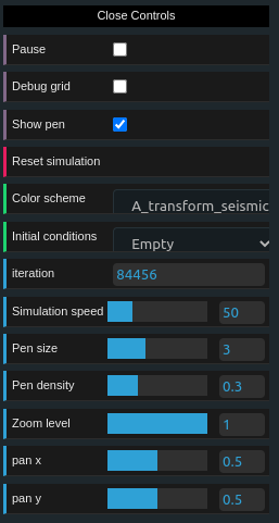
Manual

This is an interactive view of the model.

The menu on the left allows the user to change the f and k parameters of the simulation and see how they influence the reaction. It is also possible to select a preset with the drop down menu.

In the center screen the user can drop some amout of solution by moving the mouse around and clicking the left mouse button, the solution can also be removed with the right mouse button. The user can also zoom in the simulation by holding the Ctrl button and scrolling with the mouse wheel (note that there is a bug in the zoom mecanism which move the simulation around when zooming in/out).

Finally the menu on the right allows the user to tweak various parameters like the color scheme used, the speed of the simulation (which you might want to adjust proportionally to f), the initial conditions, the pen setting to add or remove the solution, etc...

Unlike the Auto tab, this simulation lets the user tweak the parameters as they want. This is a good tool to understand how each parameter impacts the simulation. A few tips to get interesting patterns:

• Don't change the f and k values too quickly, abrupt changes tend to stabilize the system very quickly.
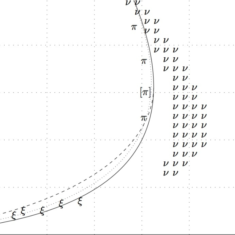
• If the simulation stabilize completely either use the mouse to add new chemical, hit r to reset the world or move fk around.
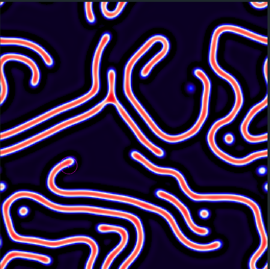
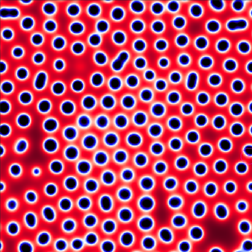
• In the selection menu on the left the orange area of the parameters map is the area which tends to produce more patterns. By moving around you'll find that there are a few different areas: the bottom left tends to produce largely chaotic patterns, a little bit higher and on the right we find patterns ressembling cells divisions, higher up are worms on the left and dots on the right with different characteristics as we go higher on the f axis. On his website Robert Munafo represents these areas like this:

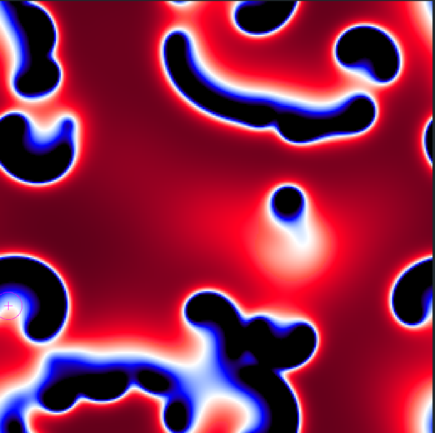
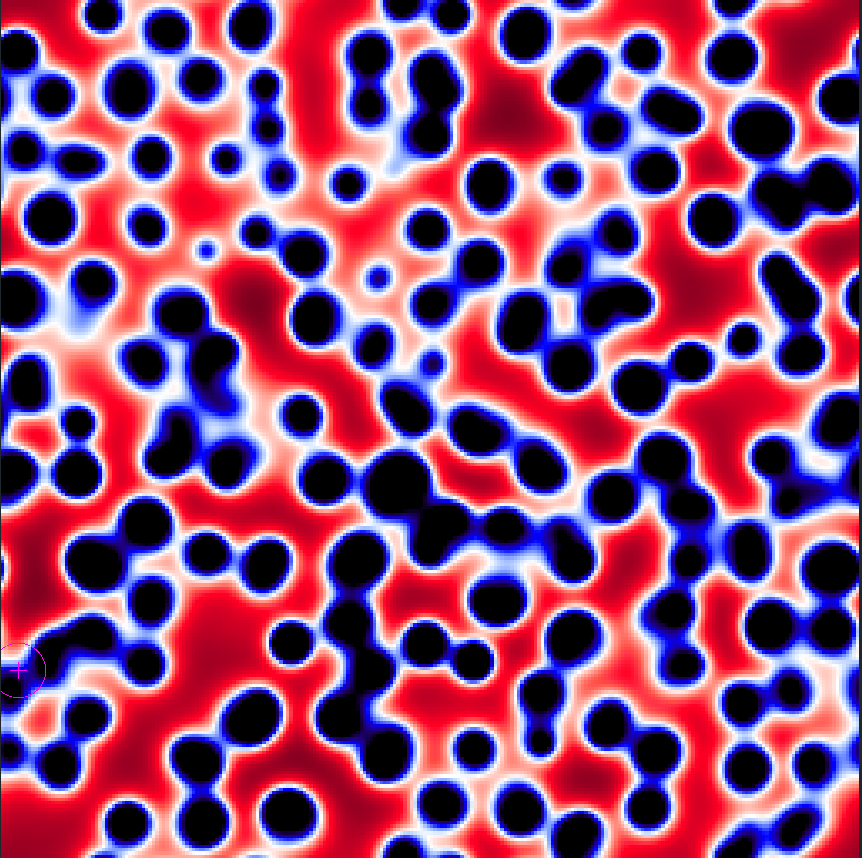
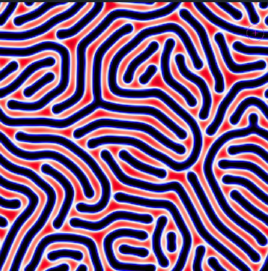
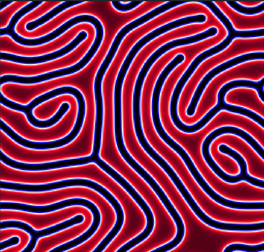
You can try to find many different patterns like the following:

Auto

This is my "artistic" stake at this simulation. My goal was to explore infinite simulation. I wanted to have a screen which would be infinitely smoothly evolving.

The f and k parameters are contiually changing to automatically generate different kinds of patterns. A mecanism also regularly regenerates some amount of solution so that there is as few stable states as possible. The user doesn't have to do anything, just load the tab and watch funny colors move on the screen.

You can use the menu on the left to tweak how fast the f and k parameters change and how much they change at each step. In this tab the fk parameters are bound to the white polygon as this is the area with the most interesting parameters classes.

There are several configurations to try out and which give various results:

• Increasing the change magnitude impacts the stability of the system. Small change magnitudes keeps f and k in a smaller area so the diversity of patterns generated is reduced, on the other hand larger magnitudes will create larger changes in the parameters space so it might create situations where the one of the chemical reacts with all of the other leaving a uniform colored texture.
• Increasing the change rate update the parameters more often which might give more time for configurations to stabilize and display all of their features.

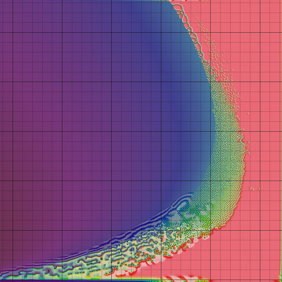
Parameters map

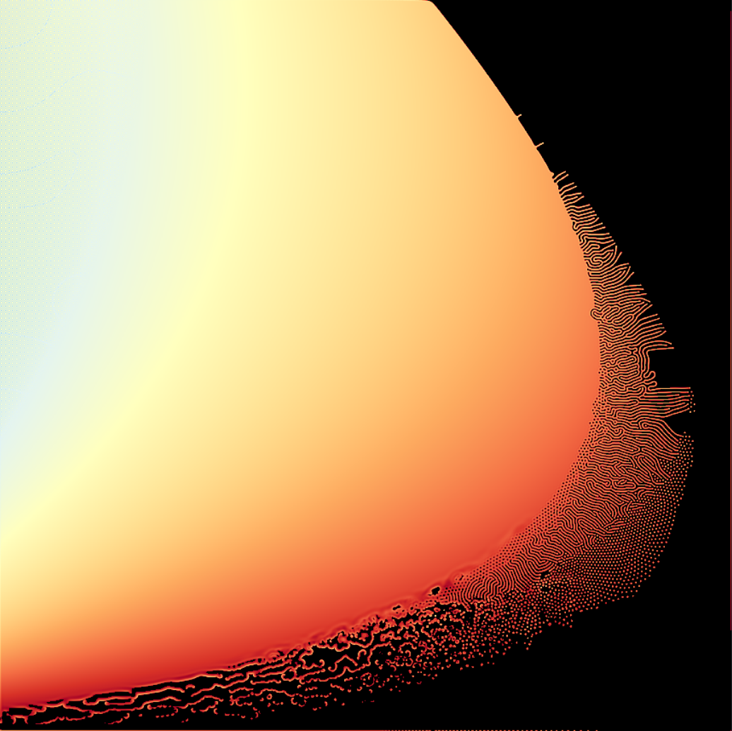
I used this tab to generate the parameters map used in the parameters selection menu. Here the difference with the other tabs is that the f and k parameters are not uniform accross the grid, they vary accross the screen to show the different possible patterns.

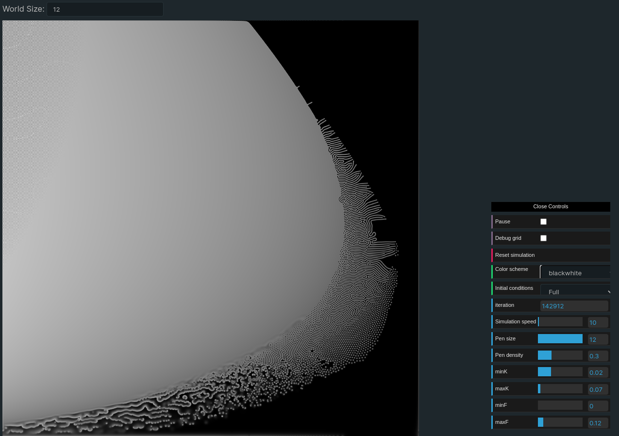
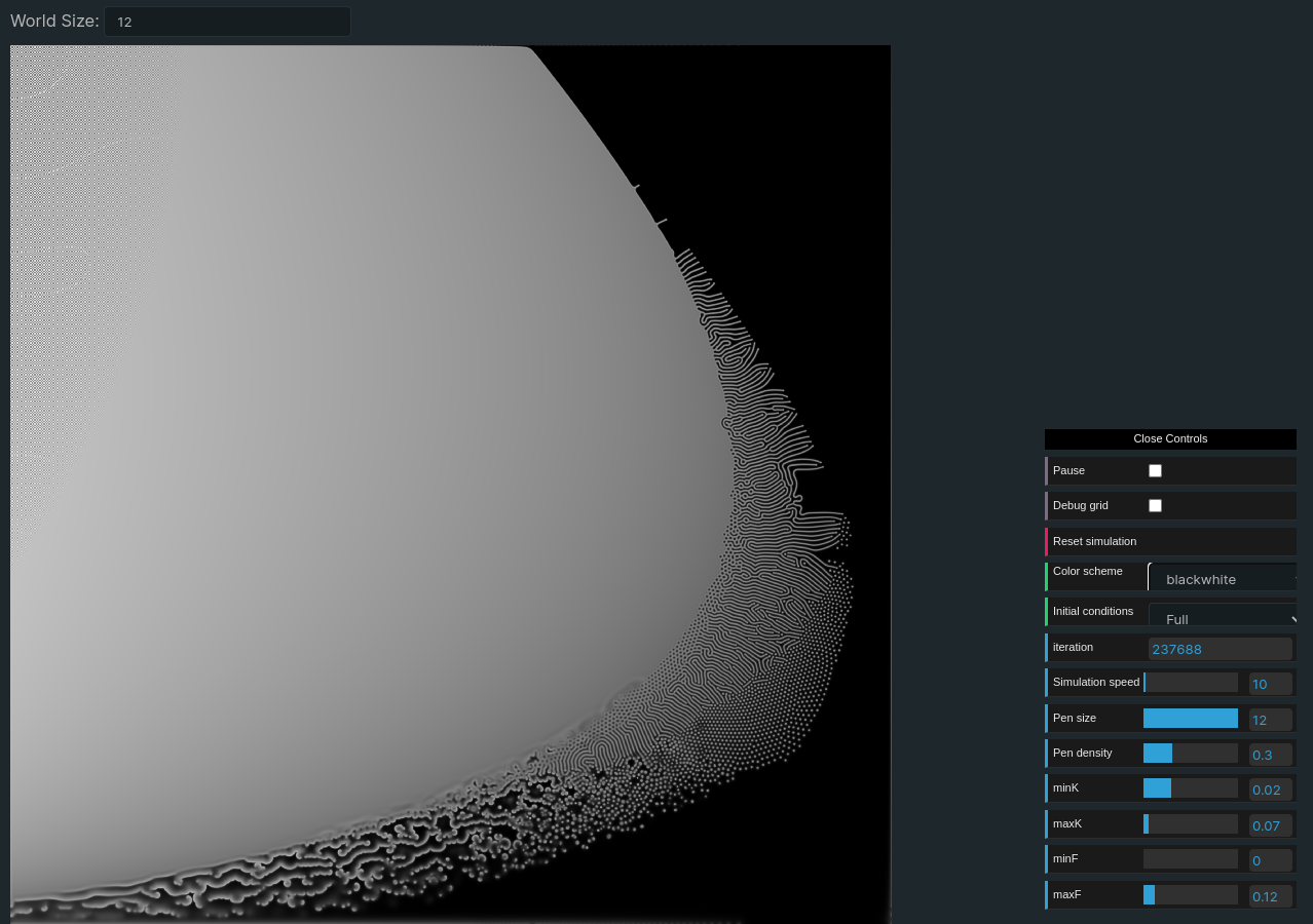
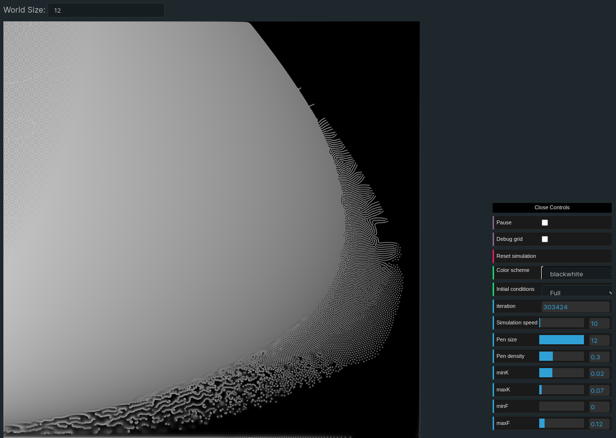
At the top of the page there is an input allowing to change the size of the underlying simulation. Increasing this parameter increases the definition of the simulation and gives a more detailled parameter map, naturally that also increases the load on the GPU runing the simulation. By default this setting is set lower than what I used to generate the final parameter map. To generate the parameters map in the fk selector of the other tabs I used a world size of 12 (which makes a texture of 4096x4096 pixels) and the simulation ran for ~140.000 iterations. I was curious to see what would happen with more iterations but it turns out the evolution is not significant after the first hundred thousands iterations:

Previous versions

It took me several iterations to get the results shown in the other tabs. This tab regroups my different iterations and a section later in this page describes the different versions.

Gray-Scott model

The Gray-Scott model is a simulation of two chemicals reacting together. Here the chemicals are named U and V.

The environement is represented with a 2D grid in which each pixel holds a level of concentration of each chemical. The simulation consist in updating the grid following these equations (picture taken here):

The chemical reaction section shows that when 1 unit of U and 2 units of V are in contact they react to become 3 units of V. The second part showing that V produces P is not really considered in the implementation, P only represents a byproduct of the reaction which is necessary for the math to work but doesn't really impacts the simulation (at least to the extent of my understanding).

The equations show 3 things:

• Both chemicals diffuse over time and the diffusion from one spot depends on the concentration of the chemical in the surrounding spots
• The chemicals react together and that impacts their concentration (which makes sense if 1 U and 2 V create 3 V then during the reaction the concentration of U diminishes and the concentration of P increases)
• f and k are respectively a "feed rate" at which we add some U and a "kill rate" at we we remove some V. This allows the model to keep evolving.

Karlsims has the clearest explaination of these equations. mrob also has a good explanation.

The way that I represents this system in my mind is as follow:

• Let's have two tanks containing the solutions one on top of the other.
• Both tanks are separated by a semi porous membrane which only allow the U solution from the bottom to go the tank above containing V.
• What we see in my simulation is the surface of the top tank while the U solution is slowly introduced to the V and both react together.

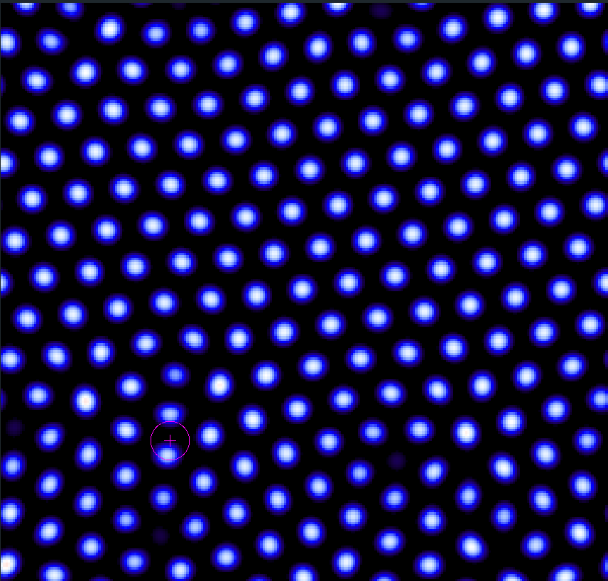
Turing patterns

The reason why this model is so fascinating is because it gives us a glance at how ordered patterns can emerge from the randomness of nature. This is related to a concept which was theorized in 1952 by Alan Turing and is named Turing patterns

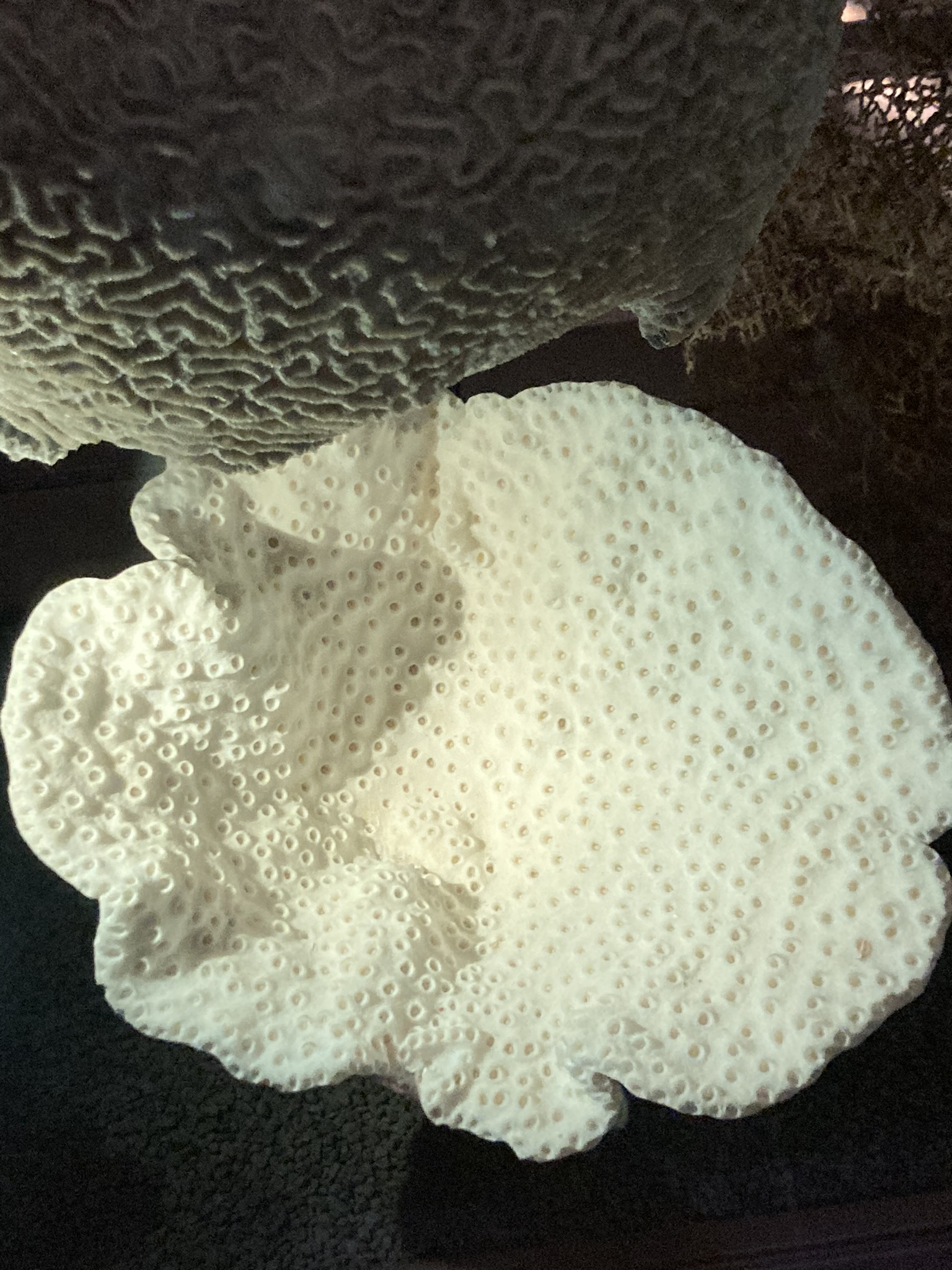
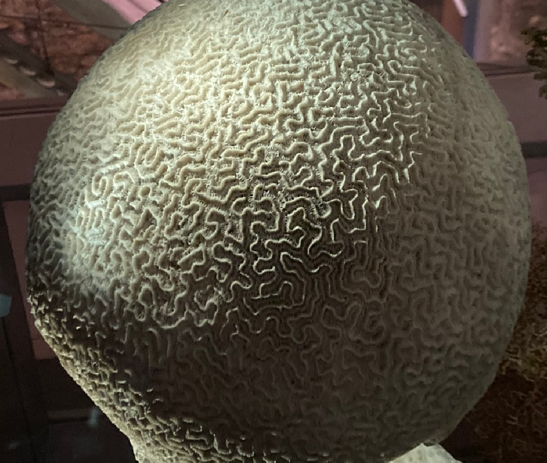
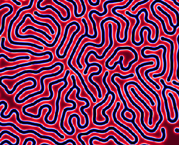
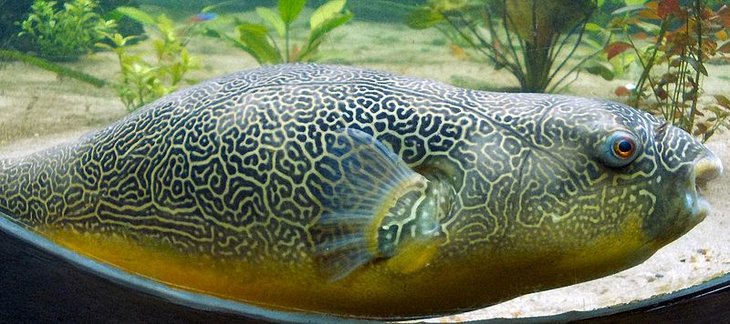
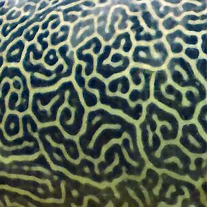
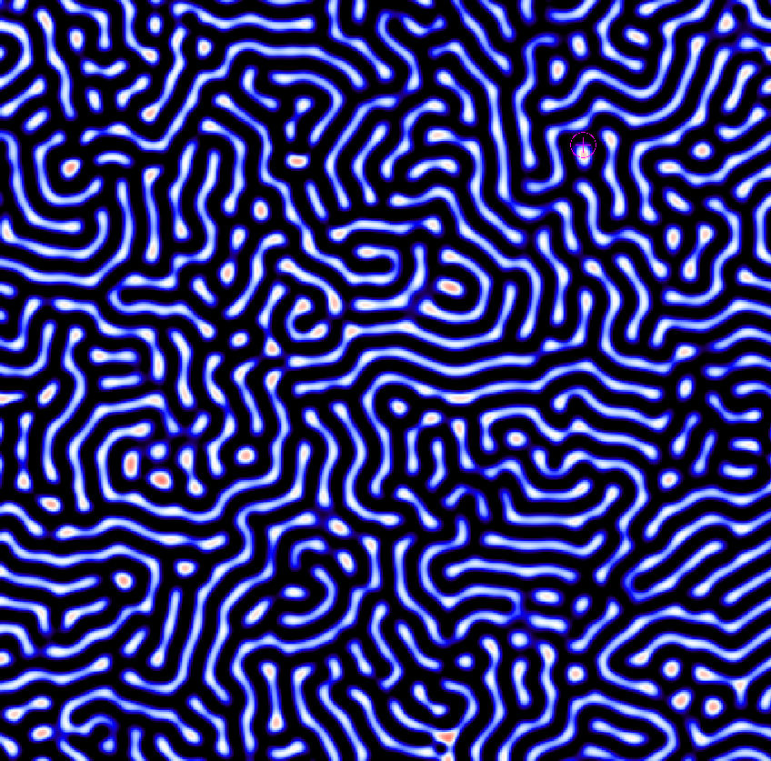
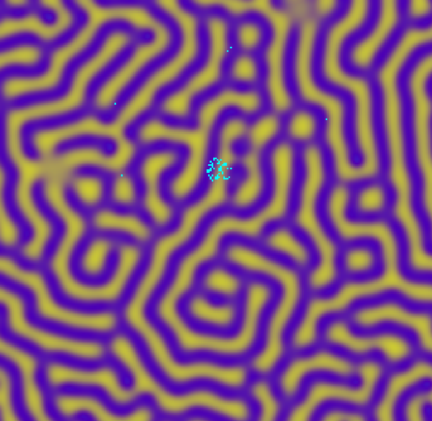
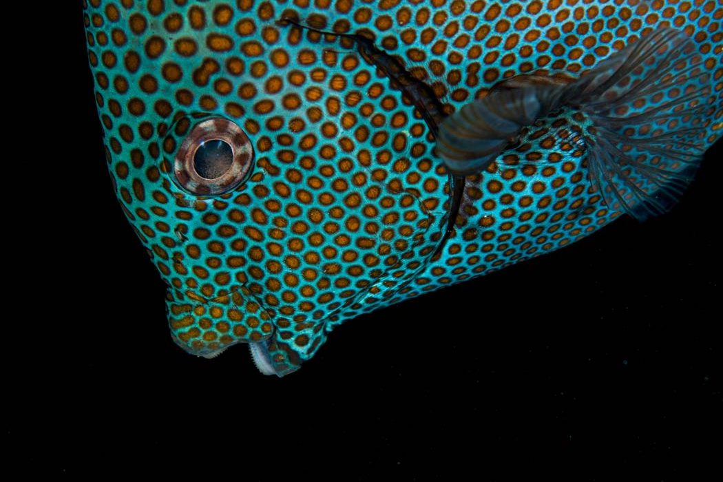
This is hard to reproduce exact existing patterns because nature is complex whereas this model is quite simple but here are a few similarities I have found:

This are two madrepora corals I took in picture at La Grande galerie de l'Évolution in Paris:

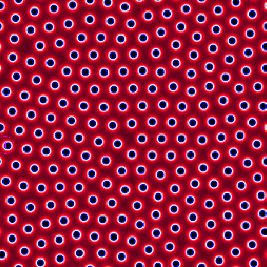
This is a puffer fish picture from wikipedia ([1] [2])

Here are some behavior ressembling to cells mitosis:

A fish from shutterstock not sure which specy this is:

Resources

Here are some resources which I found useful while making this project.

Gray-Scott model

• Karlsims tutorial about Reaction-diffusion, very good introduction and good explanation of the formula https://karlsims.com/rd.html
• Mrob list of a lot of interesting parameter classes https://www.mrob.com/pub/comp/xmorphia/pearson-classes.html#eta
• Mrob Uskate parameter space https://mrob.com/pub/comp/xmorphia/uskate-world.html
• A very good high level introduction to reaction diffusion with some great analogies with the particule approach. Lot of interesting links. https://www.redblobgames.com/x/2202-turing-patterns/
• Redblobgames implementation of the parameter map visualisation https://www.redblobgames.com/x/2203-reaction-diffusion/art/parameter-map.html
• Good schema of the experience, one clue about the color map and a parameter space graph visualisation https://itp.uni-frankfurt.de/~gros/StudentProjects/Applets_2014_GrayScott/
• A scientific paper "Spatially localized structures in the Gray-Scott model" https://royalsocietypublishing.org/doi/10.1098/rsta.2017.0375

Color maps

• General approach to color maps. Lot of visual representations of colormaps. The interesting one here is the diverging method. https://matplotlib.org/stable/tutorials/colors/colormaps.html#diverging
• A lot of colormaps implemented in glsl, I reused a few of them in my code. https://github.com/Polymole/glsl-colormap

Other implementations

• Redblobgames Various configurations with creative results.
• Robert Munafo Lots of presets to play with and a very good color picker.
• pmneila About the same set of features as Robert's implementation, with a dark theme.
• Karlsims Very good looking 3D like effect, flows applied to the whole grid and great interface.

History of the project

The code of all the versions described here is available on this project's repo on Github.

Prototyping with P5.js (v1, v2, v3)

In versions v1, v2 and v3 were prototyping to validate my understanding of the math behind the model and of the general idea of the simulation.

These versions use the p5.js framework to render and update the simulation. The world is represented by a 2D array in typescript and the update is a simple nested for loop iterating on each item of the grid and applying the formula.

The main difference between these 3 versions is the way I was updating the grid. In v1 I started with a very naive approach where I recreated the grid on each iteration. In v3 the algorithm is smarter, I create two grids when I build the world and then each update reads from one of the grids and writes to the other one which is then used by p5 to draw the canvas. This is a classical but inefficient approach to this kind problem.

With a grid of 500x500 pixels the frame rate is around 1 fps with 1 iteration by frame which isn't great. In comparison on the same machine my final version runs grids of 512x512 pixels rendered on a full screen at ~55fps with 50 iterations by frame, which is much better!

Dabbling with WebGL (v4)

With the 3 previous versions I validated I understood the model and in v4 I started to make the simulation larger by using the GPU to update the world instead of doing that on the CPU in typescript. This was my first experience with regl which is an incredibly cool framework to make working with WebGL much easier. This version was laying the fundations for my WebGL simulation: First, in typescript we generate a grid representing the world and we generate two WebGL texture where each pixel is an item of the generated grid.

For each pixel we only generate a value on the red and green channels. Each value is comprised between 0.0 and 1.0 and corresponds to the concentration of the two chemicals U and V in each discrete position of the world.

Once this is done we create two regl commands:

• The update command which is responsible for reading from one of the created texture and updating the new state in the other texture.
• The draw command which simply takes the last updated texture and draws it directly on the canvas. The texture is drawn "raw" as in the red and green channels are used directly in the shader.

precision mediump float;
uniform sampler2D prevState;    // The state of the simulation to render
varying vec2 uv;                // The position of the vertex in the simulation texture
void main() {
    vec2 state = texture2D(prevState, uv).rg;   // Read the red and green channel in the simulation
    gl_FragColor = vec4(state, 0, 1);           // Use them directly in the color
}

Adding basic controls to the simulation (v5)

Once my simulation was working properly on the GPU I wanted to add some interactivity.

It was the opportunity to play with dat.gui. This is a library which allows to easily create a graphical interface to modify the properties of a javascript object. I had already experimented with this library in my previous game of life project

In this simulation I added the following settings:

• A very crude manual selection of f and k parameters, allowing me to better grasp the impact of the feed rate and kill rate.
• Some additional presets seletions for f and k. I took these presets from the examples in Robert Munafo's extended pearsons classification. The fact that the classes I took from Robert's website were producing results similar to his own implementation was an encouraging sign that I was going in the right direction.
• A setting allowing to use different initial conditions for the world. It is useful because this version doesn't allow to modify the world with the mouse so having different starting worlds allowed me to test different f and k parameters.
• Some basic settings like the ability to pause and reset the simulation or see the current iteration number.

Using the mouse to change the world (v6)

v6 saw a big improvement in my way to handle the glsl code for my shaders: instead of writing the shader code directly in the initialization of the regl commands (as it's shown in regl's examples) I created a mechanism which allows me to write the shader code in separate .glsl files which are imported in the typescript code and then injected in the regl commands properties.

Having a better separated code allowed me to pass more uniforms to my shaders and particularly to pass the mouse state to the update shader. Now the shader takes the position of the mouse as well as the state of each mouse button as uniforms. This way when updating each pixel if the pixel is close enough from the mouse and the button is pressed we can override the new value of the pixel (and ignore the value coming from the simulation). That allows to artifically increase the concentration of one of the chemicals on specific spots of the world.

Zoom and fk selection (v7)

In v7 I focused on the UI of the application. A lot of things changed on this iteration.

Firstly I reworked the regl code and created two separate pipelines for the simulation itself and for its rendering. The simulation pipeline is basically the same one as in the previous versions.

The graphic pipeline is pretty different:

This version introduce a system where I use several texture to apply different transformations to the simulation texture before displaying it on the screen:

• Step 1 "Zoom": In the vertex shader of the graphical pipeline I pass as uniforms the state of the zoom (i.e. the zoom level and the pan on the x and y axis). These uniforms allows me to draw only the parts of the texture which are currently in a zoomed in area.
• Step 2 "Colors": To make the simulation more visally appealing the first stage takes the raw red and green channels of the simulation texture and transform them to use a wider spectrum of colors. Since regl makes the glsl code quite modular I was able to create different fragment shaders applying different color palettes.
• Step 3 "Grid": To help me debugging the implementation of my zoom mecanism I added a step which overlays a grid on the resulting texture. The goal was to have a grid with a fixed sized which would better show the resolution of the zoom.
• Step 4 "Cursor": To make the mouse drawing more intuitive I add another overlay showing the area which the cursor will drawn on.

This approach has the big advantage of keeping my code very modular and making it easier to implement the different steps. The main drawback is that it requires to keep one texture for each step of the pipeline which has an impact on the GPU. An alternative solution would be to do all the transformations in the same shader but I haven't experimented with that already and I'm not sure what are the best practices for this topic.

I also created the interface to select f and k on the parameters map. To do that, the first step was to create another type of simulation largely based on my previous experiements but where the f and k parameters are varying among the world. This way when initializing the world with small concentrations of the solutions and letting the simulation run for a few hundreds of thousands of iteration we get a nice map like this one

Some inpsiration I had for the parameters map:

• mrob
• RebBlobGames

"Auto Visualizer" (v8)

My last goal for this project was to create an infinite visualization based on the simulation. The issue with the raw simulation is that most of the parameters classes tend to create stable states after a number of iterations. Stable states are interesting to study the Gray-Scott system but they get boring quickly so I created the Auto Visualizer based on two ideas:

First the f and k parameters need to change regularly to create new patterns but they need to change slowly. A big step between two values of (f, k) often tend to destroy all the concentrations of chemicals. So reusing the menu component I created to select f and k, I added a bounding box of the values which create the most interesting patterns and then used a noise function to make the parameters vary slowly and consistenly over time.

Even when changing f and k the chemicals tends to disappear from the system so I have a mecanism which simulates the user clicking on the screen to add more chemical.